The metrics we use

Our collection of metrics fall into different categories and are designed to highlight the various aspects of an asset's performance.

To learn more about the time series data used as a basis for the metric calculation, read this article.

In the analysis and comparison advanced settings, the user has the option to choose whether the asset's close price or adjusted close price time series is used for the metrics calculations. Read this article for more information.

The snippets below use a few shorthands:

• r: the time series of (daily) returns
• period: the annualisation factor (252 trading days for an annual figure, 21 for a monthly figure)
• rf: the risk-free rate; set as an annual rate in the advanced settings and applied per trading day in the formulae below
• confidence: the confidence level, set in the advanced settings
• norm: the standard normal distribution

Each snippet is the essential calculation, with the data-handling and multi-asset machinery removed for readability.

Metrics measuring different aspects of the return of an asset.

Returns time series

Time series of returns between each day and the first day.

The return on the first day of the time series is always zero, as the anchor to compare all other days to.

returns_ts = (1 + r).cumprod() - 1   # r[0] = 0 anchors the first day at zero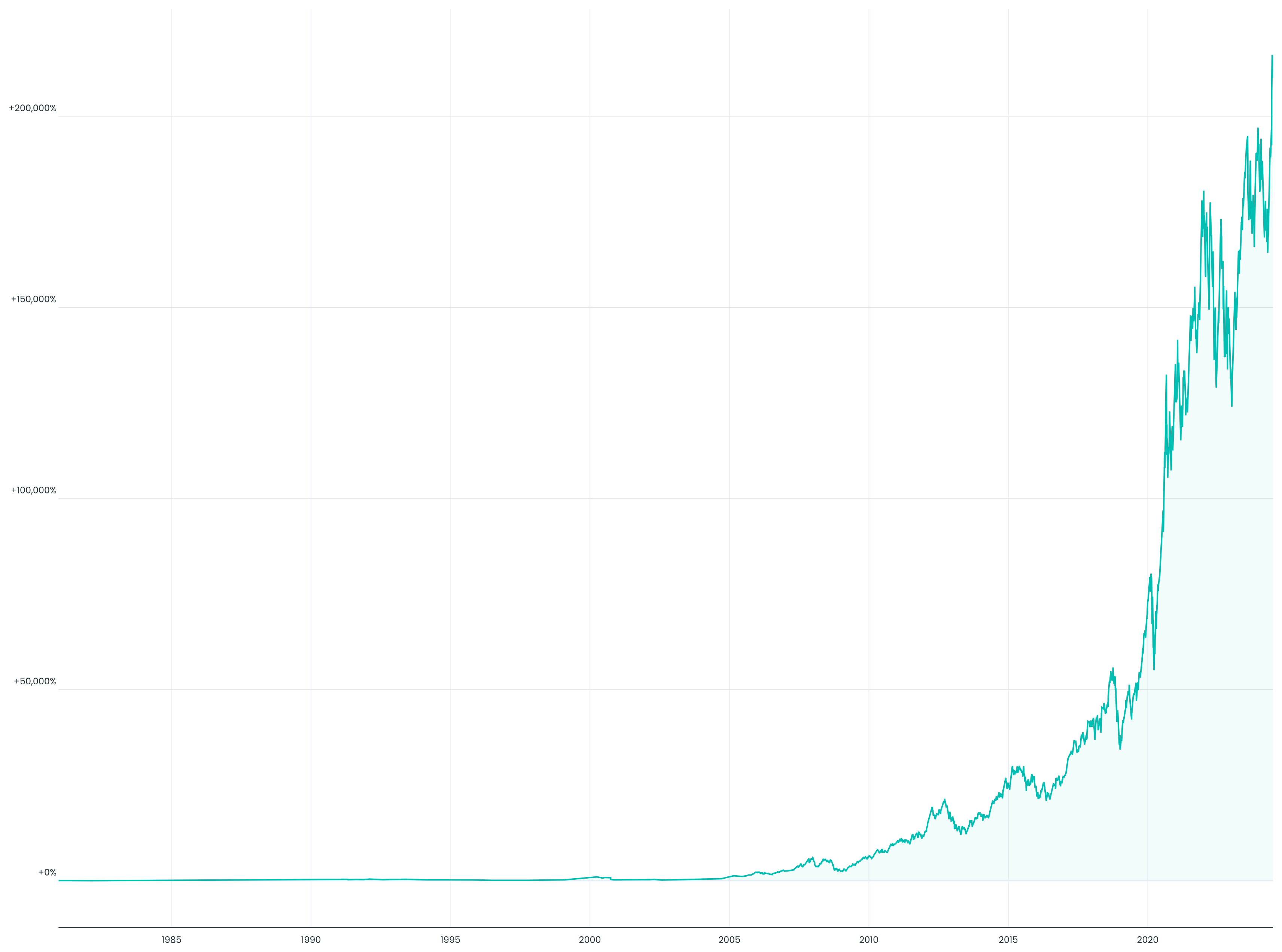

Chart for returns time series

Mean return

Mean of (daily) returns, scaled to a given period, e.g. annualised.

mean_return = r.mean() * period   # period = 252 to annualise daily returns

Return between two dates.

cumulative_return = (1 + r).prod() - 1

Period return

Cumulative return but scaled to a given period, e.g. annualised.

For example, the annualised return or CAGR of an investment between two dates 10 years apart.

n = len(r)   # number of return observations
period_return = (1 + r).prod() ** (period / n) - 1

Period yield

Difference between the return calculated with close prices vs. the return calculated with adjusted close prices, scaled to a given period, e.g. annualised.

total_return = period_return(adj_close_returns)
price_return = period_return(close_returns)
period_yield = total_return - price_return

Metrics measuring different aspects of the risk of an asset, specifically the mean risk and the tail risk.

Drawdowns time series

Time series of returns between each day and the preceding peak.

If a particular day is a new peak, the drawdown is zero. Otherwise, the drawdown is always negative.

prices = (1 + r).cumprod()
drawdowns_ts = prices / prices.cummax() - 1   # 0 at each new peak, else negative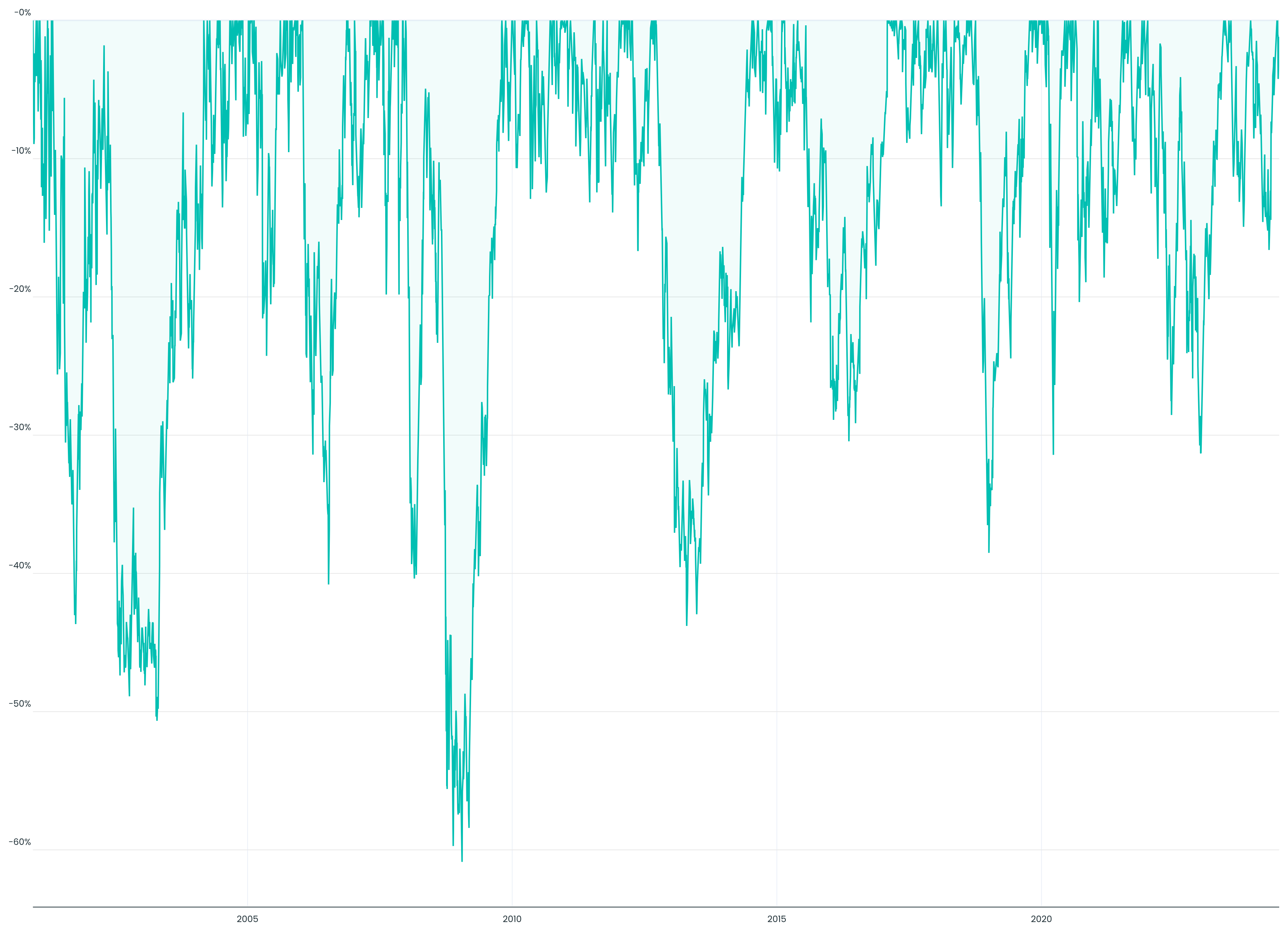

Chart for drawdowns time series

Volatility

Standard deviation of (daily) returns, scaled to a given period, e.g. annualised.

volatility = r.std(ddof=1) * sqrt(period)

Down volatility

Standard deviation of (daily) negative returns of a returns time series, scaled to a given period, e.g. annualised.

downside = r[r < 0]   # only the negative returns
down_volatility = downside.std(ddof=1) * sqrt(period)

Maximum drawdown

Standard measure of tail risk. The maximal percentage difference between a peak and a following trough in a given time series.

prices = (1 + r).cumprod()
max_drawdown = (prices / prices.cummax() - 1).min()

Drawdown

The current drawdown, as opposed to the maximum: the decline from the most recent peak to the latest value. It is the final point of the drawdowns time series—zero at a new peak, otherwise negative.

Value at risk

Hypothetical loss at a given confidence level assuming a normal distribution of (daily) returns, scaled to a given period, e.g. annualised.

For example, an annual value at risk of 10% at a 95% confidence level means a 95% probability of a loss of 10% or less in one year.

mean = r.mean() * period
stdev = r.std(ddof=1) * sqrt(period)
value_at_risk = norm.ppf(1 - confidence, mean, stdev)   # confidence = 0.95

Expected shortfall

Value at risk's sister metric, measuring the expected loss in the part of the distribution that was excluded in the value at risk calculation.

Consider this example with confidence level = 95% and period = annual:

• Value at risk = 10%: 95% probability of a loss of 10% or less in one year
• Expected shortfall = 15%: the average loss in the worst 5% of outcomes is 15% in one year

mean = r.mean() * period
stdev = r.std(ddof=1) * sqrt(period)
z = norm.ppf(1 - confidence)
z_es = -norm.pdf(z) / (1 - confidence)
expected_shortfall = mean + z_es * stdev

Metrics measuring the return of an asset in relation to the risk of an asset.

Sharpe ratio

Standard measure of risk-adjusted returns, developed by Nobel Prize winner William F. Sharpe.

An investment with a higher return than risk has a Sharpe ratio greater than one. A loss-making investment has a Sharpe ratio below zero.

sharpe_ratio = (mean_return - rf * period) / volatility   # rf = risk-free rate

Sortino ratio

Sharpe ratio but using down volatility instead of volatility as the risk measure.

sortino_ratio = (mean_return - rf * period) / down_volatility

Calmar ratio

Return per unit of maximum drawdown.

While the Sharpe and Sortino ratio use measures of mean risk in the denominator, the Calmar ratio uses a measure of tail risk.

calmar_ratio = period_return / abs(max_drawdown)

Metrics measuring an asset's performance vs. a benchmark.

Correlation

Pearson correlation coefficient between the daily returns of an asset and a benchmark.

correlation = np.corrcoef(r, r_benchmark)[0, 1]   # Pearson correlation

Beta

Measure of an asset's volatility relative to a benchmark and its correlation with the benchmark.

• Beta = 1: asset is perfectly correlated with the benchmark and has the same volatility as the benchmark
• Beta = 0: asset is perfectly uncorrelated with the benchmark
• Beta > 1: asset is correlated with the benchmark and has a higher volatility than the benchmark
• Beta between 1 and 0: asset is uncorrelated with the benchmark and/or has a lower volatility than the benchmark
• Beta < 0: asset is negatively correlated with the benchmark

cov = np.cov(r, r_benchmark)
beta = cov[0, 1] / cov[1, 1]   # covariance with benchmark / benchmark variance

Alpha

Excess return of an asset vs. a benchmark adjusted to the same level of risk.

• Annual alpha = 0%: the asset and the benchmark generate the same return when adjusting for risk
• Annual alpha = +1%: the asset generates 1 percentage point more return than the benchmark when adjusting for risk‍
• Annual alpha = -1%: the asset generates 1 percentage point less return than the benchmark when adjusting for risk

alpha = (mean_return - rf * period) - beta * (benchmark_mean_return - rf * period)

Metrics measuring the characteristics of an asset's distribution of (daily) returns.

Skewness

The skewness of the distribution of (daily) returns is a measure of the symmetry of the distribution.

A normal distribution is symmetrical and has a skewness of zero. A distribution with positive skew is asymmetrical and shifted to the left with its tail on the right side.

skewness = scipy.stats.skew(r, bias=False)

Kurtosis

The kurtosis of the distribution of (daily) returns is a measure of the tailedness of the distribution, i.e. how much "weight" is in the tails vs. the centre.

We report excess kurtosis, so a normal distribution has a kurtosis of 0. A distribution with a kurtosis greater than 0 has more "weight" in the tails than a normal distribution, while a kurtosis below 0 has less.

kurtosis = scipy.stats.kurtosis(r, bias=False)   # excess kurtosis: normal = 0